
Author: William Fletcher, Datatonic
You’ve doubtless come across recommenders before. You’ll certainly have been on the receiving end of a few. The question is, what do they look like on the inside?

In fact, there is tremendous variety – recommendation is an old problem, and was first tackled within classical information retrieval in the 80s. Since then, deep learning has inevitably infiltrated the field, and recommenders today are often designed around neural networks.
Typically, the different recommender setups are treated separately. Within a given dataset, you would look for an archetypal form and start building a recommender of that type. But instead of pruning your dataset to fit a well-studied example, are there ways to design a solution that fits your dataset? In this article I’ll suggest how you might try.
To begin, let’s recap the familiar ways.
Recommender archetypes
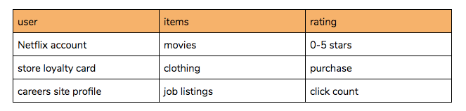
One basic recommender setup, for example the Netflix Prize problem, centres around a user–item matrix. Entries of this matrix are ‘ratings’ that a user gave to an item (movie), and some of the entries are missing.
The recommender task here is to fill in the missing ratings so that we know which movies a user is likely to rate highest when watched. These would then be suitable suggestions to make to the user if we want them to have a good time on Netflix. Naturally this idea is extremely versatile, extending to any scenario with identifiable ‘users’ and some explicit or implicit ‘rating’:
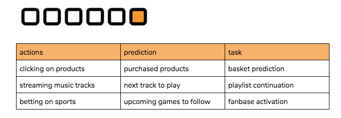
But that’s not the only task in recommendation. Another common pattern comes from trying to extrapolate a sequence of related actions, or predict some final action. Typically this might be a real-time “session” of online activity, but other examples exist for longer timeframes:
Other setups include:
- Content-based recommendation – where there exists metadata for the items and/or users – modelling the nature of the item rather than its identity. These approaches have the advantage of translating well to new items.
- Association rule mining – where co-occurrence is favoured over other signals.
- Similarity measures – for example, recommendation by selecting the most similar song to the one just played.
- Knowledge-based recommendation – where the items shown are selected by extrinsic knowledge of their aptitude (using hard and soft criteria rather than observation)
What do the archetypes above have in common?
Well, the task is always to recommend. That is, to take a collection of potentially interesting items and pick out the best. Described like this, it’s essentially a search problem: to display the most relevant content for the query. But... what is the query?
The state of search
This is where we turn to the latest in web search for clues.
When you make a search request at google.com, there is more going on behind the scenes than simple document retrieval. In fact, Google links to a page explaining the signals it uses to enhance your query.
It almost seems as if they know what to show you before you even ask for it…
In case I was too subtle just then, I’ll restate my point: recommendation is search without an explicit query. Instead of processing a text input to deduce intent, we rely only on contextual clues such as when and where the user is right now, their personal profile, and recent activity. Overloading the term, we shall refer to all of this together as the ‘query’ of recommendation. Inside this search framework, we have the following channels to design and exploit:
Just as with smart web search, different contextual signals may contribute in different ways to the final results of a recommender system. While it is certainly possible to set up a super-mega-ultra all-in-one solution, why bother? Is it worth the struggle to build a model that uses everything at once, or conversely, treats the inputs totally separately and individually?
Extension and Combination
The pragmatic idea of a composite recommender is not this author’s to claim. In a 2002 paper by Burke, seven answers are given to the relatively benign question of how to form a “hybrid” from two or more archetypal recommenders:
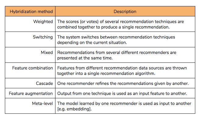
Yes, these techniques were intended to apply to hybridizing existing recommenders, but the principles apply just as well to building a modular multi-input recommender from scratch.
Although – caveat – the first four approaches do not offer a real response to the question posed at the end of the last section. Only the last three (“cascade”, “feature augmentation” and “meta-level”) have any flexibility.
To illustrate the principles of modular recommender architecture, we’ll now examine a dummy dataset with all the typical tables you might expect when tasked with building a recommendation engine. We’ll then show how this approach might help make a manageable ML project out of an otherwise daunting proposition.
Data
It helps to consider that there are 4 types of source metadata before thinking about derived information:
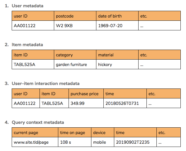
From these sources flow all useful truth. It is the job of the data scientist to extract it, and the data techniques applied can be drawn into largely distinct groups, illustrated on the below diagram.

The first level of information mining is association, with the intent of binding one entity to another by similarity or co-occurrence of entries in a table:
- from User metadata
(user, user) → similarity - from Item metadata
(item, item) → similarity - from User–item interaction metadata
(user, item) → affinity
(item, item) → association
(user, user) → associationSecond, there is feature engineering, with the intent of capturing information to be used in later efforts. Features are often transformations or aggregations of data in source tables:
+ Item features
= user-supplied metadata (e.g. tags, comments)
= aggregated user interactions
= aggregated user features
+ User features
= aggregated item interactions
= aggregated item features
+ Contextual features
= item context (novelty, trending etc.)
= user context (recent activity, past sessions)
And finally there is modelling – constructing additional information through machine learning, supervised or unsupervised:
- Item embeddings
- User embeddings
- Imputation
- Recommendation
Constructing complex recommenders
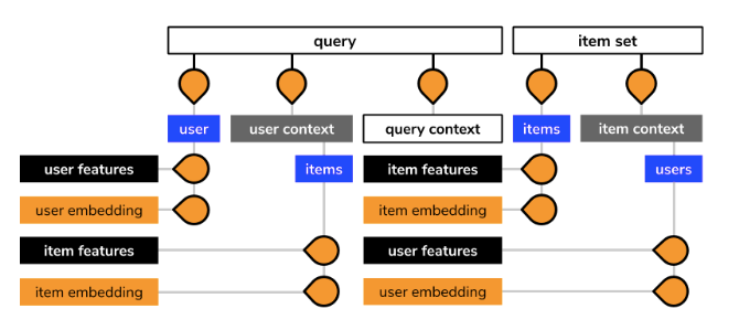
Under this framework, it becomes easier to lay out how to assemble an advanced multi-input recommender. It may help to think in terms of the operations available to us.
Start with the definition of the recommender problem:
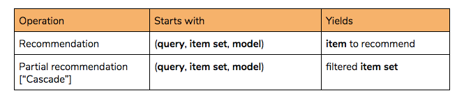
To this add some elementary operations to obtain features:
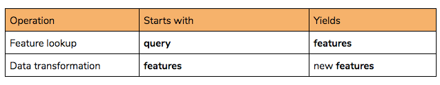
And lastly some elementary operations for modelling:
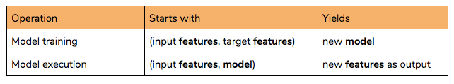
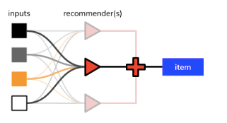
Model training may involve any combination of inputs and outputs from the features described so far. Using or obtaining an embedding (“meta-level” hybridization) is illustrated with orange in below diagram. And “feature augmentation” is simply a matter of chaining the process into another model.
So, with model combination abstracted away, the ‘irreducible unit’ of modelling is this:

The final layer
At this stage we are back in line with Burke’s work. Having dealt with “meta-level”, “feature augmentation”, and “feature combination” types of hybridization in the last section, we are left with the relatively simple “weighted”, “switching”, “mixed” and “cascade”, all of which shall simply be represented without comment by the diagram from earlier:
And just like that, we’re done.
Concluding remarks
In this post, I’ve deliberately avoided the particulars of neural network architecture, feature engineering, or other mathematical choices that will inevitably be just as rich a field of variation as the concepts described above. My hope is that any readers who have enjoyed or appreciated this journey through data space will put careful thought into the craft of advanced recommenders, and consider intelligently the relative merits of increased complexity at each scale. Deep learning can sometimes overwhelm by its scope and pace, but its practice should always aim to address the real problems – this article contributes by making more explicit some decisions that are often taken implicitly.
Good luck, and happy recommending!